The Geometry
Behind Normal Maps

I first ran into tangent space while learning about normal mapping. It was described as this in-between space that connects surfaces and UVs, something you need to make lighting work. Nobody really explained what it was. Tutorials showed math and shader code snippets, but none of them answered the real question: what is tangent space and why does it exist at all?

When I first learned about normal mapping I didn’t care as long as the normals looked right. But while working on mesh processing for VGLX that answer stopped being enough. I wanted to understand what those tangent vectors meant, not just how to compute them. What geometry were they pointing to? What was this “space” actually describing?

Eventually I realized the answer wasn’t mysterious at all. Tangent space isn’t a rendering trick. It’s a geometric structure that appears any time a surface has a parameterization. I just hadn’t connected the dots before.

When we define tangent space using UV coordinates, it becomes the bridge between the flat world of texture coordinates and the curved world of 3D surfaces. Once you see that connection, normal mapping suddenly makes perfect sense.

In this article I’ll take tangent space apart piece by piece: what it really is, how it emerges from UVs, how it’s computed, and how it forms the foundation for normal mapping and other techniques that depend on local surface orientation.

The Anatomy of Tangent Space

Tangent space isn’t a global coordinate system. It’s a local frame built independently at every point on a surface. Each point has its own small world, a tiny patch of geometry defined by the surface itself. The tangent plane is that world’s foundation: a flat approximation that captures how the surface behaves locally and where the space gets its name.

Every point on a smooth surface has a tangent plane defined by its normal vector. We can see the same idea in two dimensions: to find the normal at a point on a curve, we first take its tangent line, then rotate it ninety degrees. The tangent plane is the 3D version of that relationship.

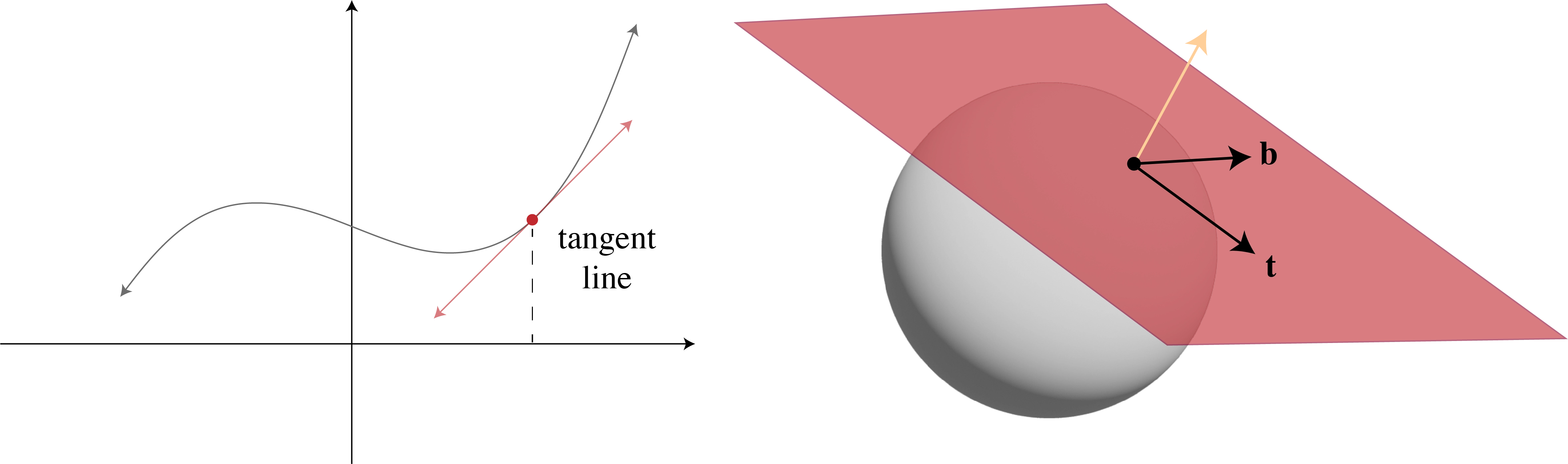
Tangent plane at a point on the surface with two tangent vectors lying within the plane.

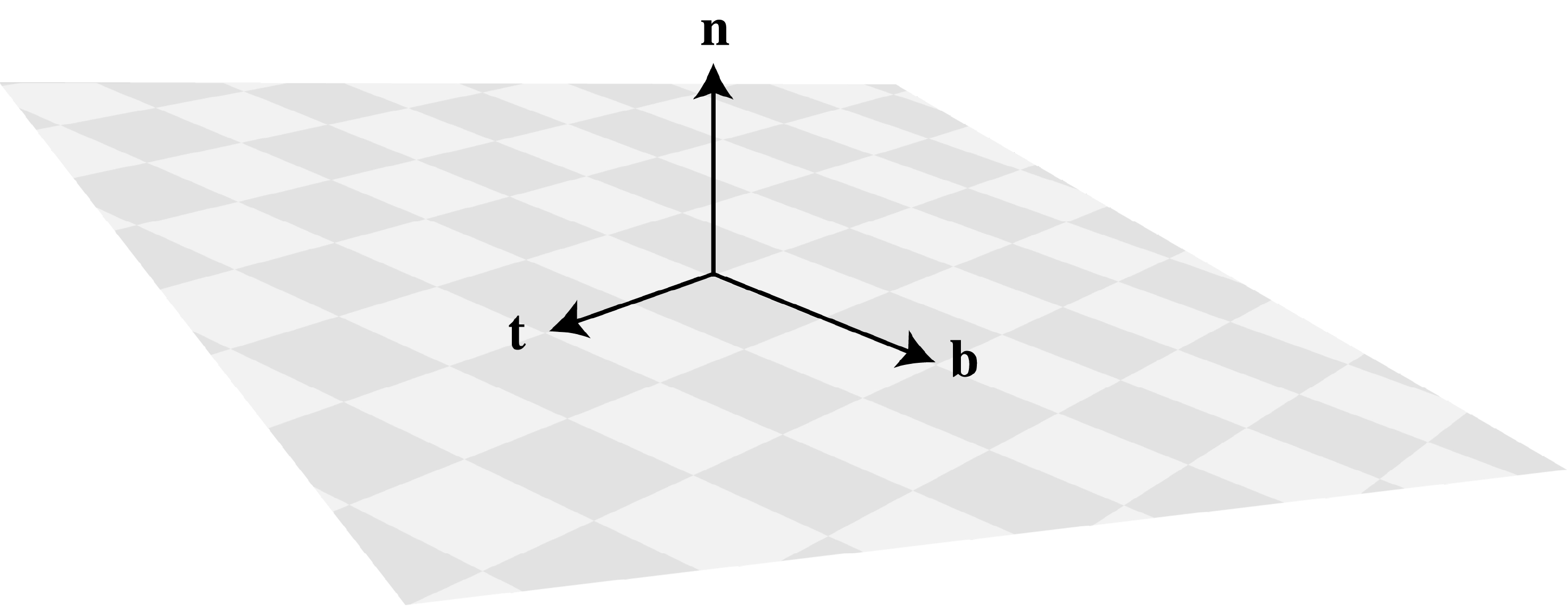
Vectors that lie on this plane are called tangent vectors. We can pick two perpendicular directions within the plane that together with the normal form an orthonormal basis: a local coordinate frame on the surface that we call tangent space.

Tangent space lets us express directions, derivatives, and transformations relative to the surface itself rather than the world. That's important because most shading computations depend on directions defined locally: light hitting a surface, a normal perturbation from a texture, or the direction of anisotropy.

But before we can use it we need to decide how to orient that local frame. For that we typically turn to the surface's UVs.

How UVs Define Orientation

When people say "tangent space" in the context of computer graphics, they almost always mean a specific orientation of that tangent frame derived from UV parameterization.

A UV map gives every point on a surface a pair of 2D coordinates. These coordinates define how textures are applied, but they also do something more subtle: they tell us how movement in 2D texture space translates to movement along the surface.

Think of UVs as a coordinate grid draped over the mesh. Moving in the U direction means sliding along one axis of that grid and moving in V means sliding along the other. Those movements correspond to real 3D directions on the surface and those directions are exactly what defines the orientation of tangent space in practice.

The tangent directions follow the UV axes matching how texture coordinates move across the surface.

This connection between texture coordinates and surface geometry is what makes tangent space so useful: it anchors the surface’s local frame to something a shader can sample. The math for building that frame comes directly from this relationship.

Constructing Tangent Space

The tangent vectors that define the orientation of the tangent frame are called tangent and bitangent and they describe how texture coordinates move across the surface. Together with the normal vector these directions form the matrix which transforms any vector expressed in tangent space, such as a normal from a normal map, into the surface's coordinate frame at that point.

Assuming the normal is known we need to find the tangent vectors and to complete the matrix. The only data that links texture space to surface space are the UV coordinates. If we have those we can say that every triangle on a mesh exists twice: once in surface space, and once in UV space. These two versions describe the same region expressed in different coordinates. This relationship defines the directions we are looking for.

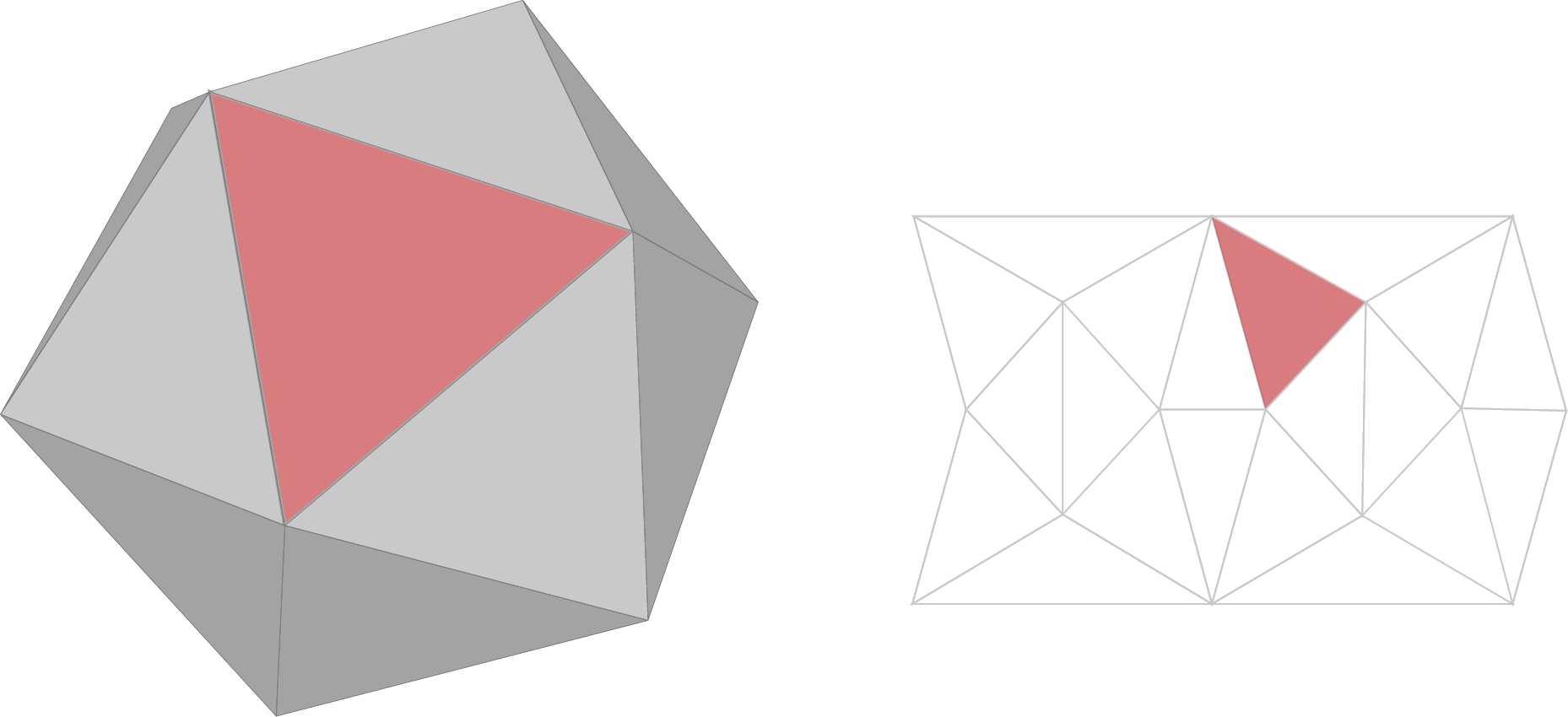
Triangle shown in surface space and its corresponding triangle in UV space (texture map).

Finding a transformation that maps directions in texture space to their corresponding directions on the surface is what it means to find the tangent vectors. This transformation can be represented as a matrix¹ whose columns are and , the directions that describe movement on the surface when or change by one unit.

We can start by defining this relationship for a single edge. Take a triangle defined by three points in 3D space, and their corresponding texture coordinates . We can compute one edge of the triangle in surface space and its corresponding edge in texture space:

These two edges describe the same portion of the triangle. We can express how the edge in texture space maps to its surface space counterpart with the following equation:

In this equation, represents a linear transformation that maps edges from texture space to surface space. Its columns are the tangent vectors that define the orientation of tangent space and form its local basis together with the normal. But one edge pair isn’t enough to find these vectors. We need another pair that shares the same orientation.

We can compute and by following the same pattern we used for the first pair, and combine everything into a single matrix equation:

This form captures both edges, giving us enough information to solve for the tangent vectors and by multiplying both sides by the inverse of the UV matrix²:

This gives us the tangent vectors we’re looking for to construct the matrix, but there’s one more thing we need to do before our tangent frame is complete.

Tangent vectors aren’t guaranteed to be perpendicular. UV maps are rarely uniform. Unwrapping a curved surface onto a flat plane introduces stretching and compression that can cause the tangent vectors to drift slightly away from the normal.

We need an orthonormal basis for stable lighting: all three axes must be perpendicular and of unit length. Assuming the UVs are mostly continuous and locally smooth, these deviations are small and can be corrected by orthogonalizing the tangent frame using the full Gram–Schmidt process. This ensures that the tangent and normal vectors remain perpendicular and normalized:

Since the normal is of unit length we can project the tangent vector onto it using the dot product . This gives us the component of that lies along the normal. By subtracting that projection from we remove any part of the tangent that isn’t confined to the surface leaving a purely tangential direction. We then apply the same process to the bitangent by removing its components along both the normal and the corrected tangent.

Finally, we normalize both tangent vectors which together with the normal form an orthonormal basis that defines the tangent frame. Packed together they make up the matrix:

Constructing and storing the full matrix for every polygon in real time isn’t practical. It’s also unnecessary to store both tangent vectors. The typical approach is computing the tangent and the handedness sign once per vertex during asset import or mesh preprocessing³ and store them together as a vec4 vertex attribute. The xyz components hold the tangent direction and w holds the sign. We then reconstruct the bitangent at render time:

The sign is required because flipping the UVs horizontally or vertically inverts one of the tangent-space axes. When that happens the handedness of the tangent frame reverses and the determinant of the matrix becomes negative. Computing the sign is therefore equivalent to evaluating the sign of the determinant. We can get the determinant of a matrix using the triple-scalar product:

With the tangent frame defined per vertex, we can now use it to translate normal directions stored in a texture into directions on the surface.

From Tangent Space to Normal Mapping

Normal mapping shares more than a storage and retrieval mechanism with texture mapping. It solves the same problem. Real-time meshes are low-resolution because every vertex adds cost and fewer vertices mean less geometric detail.

If we could afford a polygon for every pixel we wouldn’t need textures at all. But we can’t so we cheat. Textures give fragments access to data we can’t store per vertex. In normal mapping that data is surface orientation.

A normal map stores those orientations as colors. Each texel encodes a normal vector using its RGB channels mapped to XYZ. The blue channel dominates because most normals point roughly outward from the surface. A normal map is tinted blue for that reason.

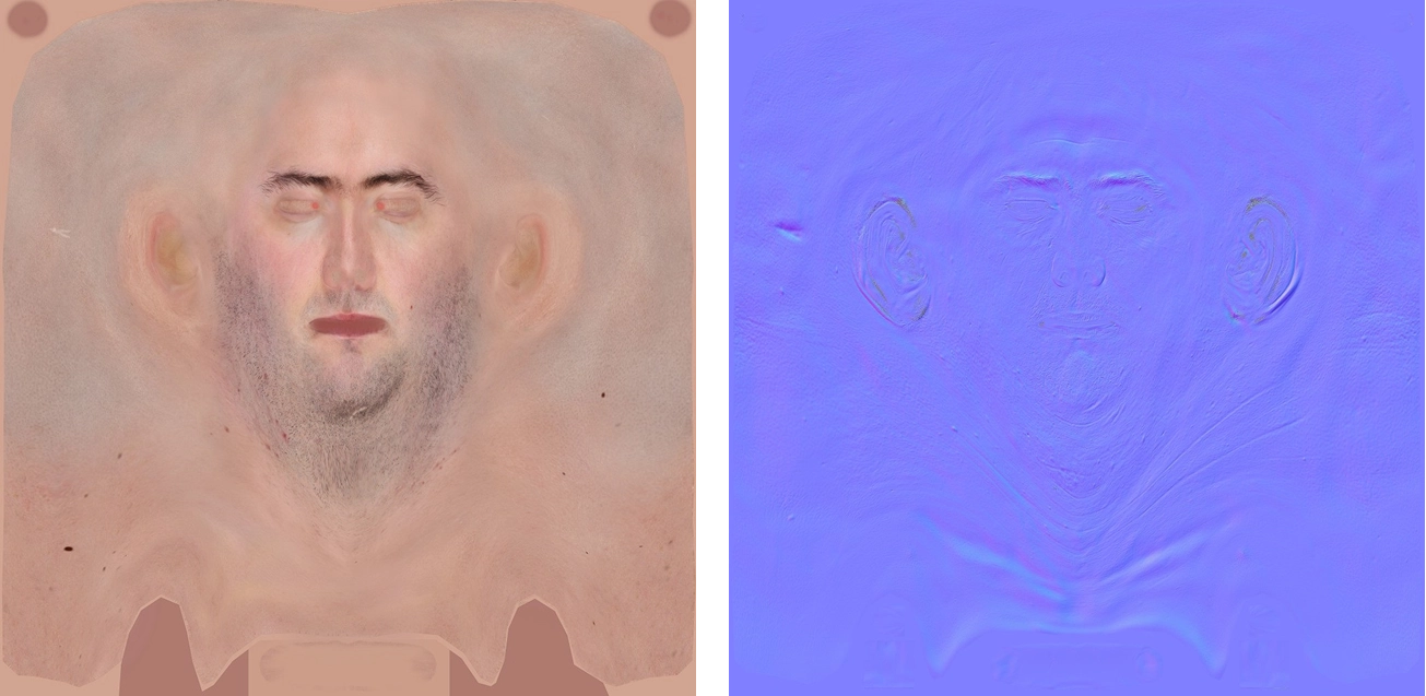
Normal map on the right tinted blue because most normals point outward.

These per-pixel normals replace the interpolated vertex normals letting lighting respond to fine details that aren’t present in the mesh.

Each texel in a normal map represents a direction in local space. We sometimes say that each texel stores a direction in tangent space in the same way that surface positions in local space are said to be in model space. The name defines the frame these values are expressed in and in the previous section we derived the function that transforms them into this frame: the matrix.

Assuming the tangent vector and handedness are stored as vertex attributes, we can reconstruct the matrix in the vertex shader:

in vec3 a_Normal;
in vec2 u_TexCoord;
in vec4 a_Tangent;
 
out vec2 v_TexCoord;
out mat3 v_TBN;
 
uniform mat3 normal_matrix;
uniform mat4 model_view;
 
void main() {
  vec3 normal = normalize(normal_matrix * a_Normal);
  vec3 tangent = normalize(model_view * a_Tangent.xyz);
  vec3 bitangent = cross(normal, tangent) * a_Tangent.w;
 
  v_TexCoord = u_TexCoord;
  v_TBN = mat3(tangent, bitangent, normal);
}

The tangent vector is transformed by the model-view matrix. Some sources say to use the normal matrix but that’s incorrect. Tangents lie on the surface while normals are perpendicular to it so each must be transformed differently.

The transformed tangent works well in most cases but under non-uniform scaling it can introduce slight angular drift. In practice this is often negligible but if precision matters re-orthogonalize the tangent against the normal before computing the bitangent.

Once we reconstruct the matrix in the vertex shader we can use it in the fragment shader to transform normals sampled from a texture into the same coordinate frame as the surface⁴.

A normal map stores directions as RGB colors in the range . To interpret them as signed vectors we remap that range to by scaling and shifting:

This converts the stored color values into normalized directions. Without this step all normals would point into a single quadrant of tangent space producing incorrect shading.

in mat3 v_TBN;
 
uniform sampler2D normal_map;
 
void main() {
  vec3 nt = texture(u_NormalMap, v_TexCoord).rgb  * 2.0 - 1.0;
  vec3 normal = normalize(v_TBN * nt);
 
  // Continue with lighting...
}

Normal maps are only half the story. They depend on the tangent frame we built earlier. If the tangent basis isn’t generated or interpolated consistently the surface won’t match the texture that defines it. Seams appear, highlights break, and the illusion falls apart. Combining the normal map with accurate tangent frames brings low-polygon models to life revealing fine detail and form that aren’t really there.

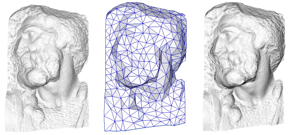
From Paolo Cignoni: the original high-resolution model (left) is simplified to a low-poly mesh (center). By transferring detail into a normal map, the low-poly version (right) recovers nearly all the visual complexity.

The process described here follows the same principles as MikkTSpace, the standard used by most tools and engines to keep bakes and renders in sync. It defines how to build, average, and orthogonalize tangents, how to store the sign, and how to reconstruct the bitangent in the shader so the lighting behaves the same everywhere.

By now the picture is complete. Tangent space gives each point on the surface its own coordinate system. UVs define how that system is oriented. The matrix connects it to the shading.

Normal mapping doesn't fake bumps. It describes how the surface would curve if it had more polygons. Shading reacts the same way because light only cares about direction, not depth. At shallow angles the illusion breaks. You can see that surface detail is missing. But viewed head-on the lighting reacts as if every point on the mesh had its own direction capturing every bump and groove.

The same idea drives everything that uses a parameterized surface. Anisotropy, triplanar projection, detail normals, even displacement mapping, all build on the same translation between textures and surface space. Once that connection clicks what seemed like a trick becomes geometry. Tangent space isn’t a feature of shading. It’s part of how surfaces exist.